Drone Mapping for Environmental Conservation

Conservation Drones in Nanaimo, BC

Drones are a powerful tool for environmental conservation. A few short flights and several hours of collecting ground control points with a GPS unit can produce fine-scale spatial data that provides environmental managers with the best data possible for prioritizing and planing restoration and conservation projects. 

Ducks Unlimited (DU) approached Smart Shores in April 2018 to conduct a field demonstration to DU staff from across western North America that would showcase drone mapping techniques and capabilities for conservation work. This post summarizes our presentation to DU staff and provides an example of the kinds of data that can quickly be produced using drones. 

Conservation Drones in the Nanaimo Estuary

This project took place in the Nanaimo estuary, just south-east of the City of Nanaimo, British Columbia. The Nanaimo estuary is made up of inter-tidal mud flats and a historic farm  that was converted back into a salt marsh as part of conservation efforts by Ducks Unlimited and the West Coast Conservation Lands Management Program. This estuary provides critical habitat for waterfowl and fish, including salmon. It is a sensitive ecological reserve and a wildlife permit is required for access and use of the site. It is also within the Nanaimo Airport control zone. We received a wildlife permit to access the site and coordinated our flight with Nanaimo Air Traffic Control. 

Drone Mapping Results

We constructed ground-point verified GIS deliverables using a process called photogrammetry (the science of making measurements from images). This involved flying a drone (UAV) in a grid pattern over the target area, distributing and measuring ground control points with a Trimble R10 GPS unit, processing the data into GIS deliverables (using Agisoft Photoscan Pro), and validating these in external software (QGIS). Photos for this project were collected by a DJI Phantom 4 Professional drone at an altitude of 120m (400ft). We performed a second flight for part of the estuary at an altitude of 50m (170ft) to provide comparative data in higher resolution. We collected data on April 17th and produced a point cloud, digital elevation model (DEM), orthmosaic and interactive 3D site tour for an in-field presentation on April 26. 

Point Cloud

Each point in a point cloud represents a point in space that was reconstructed using the process of photogrammetry and calibrated using known ground control points. Each point contains spatial coordinates (X,Y,Z - or - lat, long and elevation) and RGB (red, green, blue) colour codes. When viewed in GIS or other compatible software the point cloud appears as a 3D model of a survey area.

The point cloud produced for this site contains 430 million points, or 331 points per square metre (10.7 sq.ft.). This point density is much greater than LiDAR, with typical LiDAR point densities ranging from “sparse” point clouds with 1 point per square metre  to “extremely dense” clouds with 20+ points per m2. The dense point cloud produced using photogrammetry for the Nanaimo estuary allows for the identification of fine-scale landscape features such as individual rocks, logs and plants that are not possible using LiDAR. 

Digital Elevation Model

Digital Elevation Models are created by connecting each point in the point cloud to its neighbours, producing a raster file with a contiguous surface. The resolution of the DEM was 6.2 centimetres. That is, the DEM resolution is high enough resolution to identify and measure elements as small as 6.2 centimetres in size, such as fist-sized rocks.

Each pixel of the DEM contains a value for its horizontal and elevation position. To produce the above image, we created a colour palate that differentiated features below the vegetation line in the salt marsh with features above. In this case, vegetation was not observed below ~0.4m elevation. Therefore, all features at and below 0.4m elevation were coded blue, becoming darker every time elevation decreased by 10cm. All features 0.41m and above were coded green, becoming darker with every 10cm increase in elevation. Higher elevation features, like bushes, were coloured yellow, and the highest elevation features (trees) were coded red.

A high-resolution DEM enables the identification and measurement of fine-scale landscape features including driftwood, small creeks, old irrigation channels and stones. It also allows land managers to identify and plan for the impacts of sea level rise. In a relatively flat area like an estuary 10-20cm of sea level rise can have a serious impact on habitat and being able to predict sea level rise impacts is a conservation priority. 

Orthomosaics

An orthomosaic is a large photo-stitch where all the photos are stitched together in such a way that the viewing angle is always from nadir (i.e. straight down). This is also known as a georeferenced ortho-rectified image. Each pixel in an orthomosaic contains horizontal (X,Y - or - lat,long) coordinates, but no elevation data. To obtain elevation data, an orthomosiac must be overlain on a DEM. The orthomosaic for the Nanaimo estuary is 3.1cm resolution, enough to see and measure footprints. For example, the two pairs of footprints in the image below average 27cm and 35cm in length.

Validating Drone Maps

High-resolution data is most valuable when it is also high precision. That is, when the coordinates for each pixel of landscape data closely match the coordinates of the real- world space they represent. High-resolution data enables fine-scale monitoring of change over time and allows for precise planning and verification of restoration work.

The data produced for the Nanaimo estuary are very precise (see Table 1, below).

Table 1 - Precision and Resolution

We used 50 ground control points to calibrate the model. That is, we entered the known locations and coordinates of these points into the processing workflow to scale the model and set the coordinates to the desired units. These points were measured using ground targets and a GPS unit. We then used an additional 68 ground points collected by the same  GPS to validate the model by comparing the points collected in the field to the projected coordinates for the DEM. The error (the difference between the actual and the projected points in the model) is reported above as the model precision.

Ducks Unlimited and the West Coast Conservation Lands Management Program, the managers of the site, expressed an interest in assessing how well a photogrammetric model represents the ground surface elevation and how this compares to LiDAR. This is because LiDAR, a laser-based data collection system, can penetrate vegetation when there is sufficient space for a laser pulse to reflect off of vegetation, hit the ground, then reflect back up, off vegetation, and return to the sensor. Photogrammetry cannot represent the ground surface beneath vegetation as well as LiDAR because it is limited to visible light.

We assessed the ability of photogrammetry to represent the ground surface elevation by completing two additional survey transects of 25 GPS points each (5x5 grid ~10m spacing); one in open and sparsely vegetated ground, and the other in very thick, dense grass.

The first transect, on bare earth and sparse vegetation had a vertical error (precision) of 3.5cm with a standard deviation of 2.7cm. This was an improvement on the average of 4.8 cm (St.Dev. 3.4cm) for the entire estuary. The second transect, in very thick, dense grasshad a vertical error of 12.2 cm (St.Dev. 3.6cm). This was roughly 2.5 times greater error than the first transect. However, the vegetation had a uniform height of roughly 15cm in our sample area. The consistent difference between the measured ground surface and projected elevation of the DEM over dense grass suggests that the DEM error relative to ground points was not error per se, but rather a consistent measure of the average vegetation height.

A LiDAR-derived DEM of this site was not available so direct comparisons between our ground survey data and LiDAR data was not possible.

One concern often raised with photogrammetry is that areas with different reflectance, like shadows or bright spots, may create errors in elevation data. Because of this, it is important to minimize the effect of surfaces with different reflectivity by selecting the appropriate camera settings and maintaining them throughout a flight over a given area. Avoiding high glare and high-contrast images can help produce better results.To assess how well camera settings can reduce potential error we measured points on a variety of surfaces and compared the coordinates of the GPS points collected in the field with the projected points in the DEM. 

Surface Reflectance

For this demonstration, we used six GPS points  to validate the model’s precision under conditions of differing surface texture and reflectance (see above image). These six points are shown in red, with white arrows. Each point represents a different surface including: a metal bridge, grass in shadow, grass in direct light, wet mud, dry mud, and light coloured rocks. The average vertical error of these points is 3.3cm with a standard deviation of 2.4cm. This low error across different surfaces with varied reflectivity demonstrates that it is possible to control for the reflectance of differently illuminated surfaces with a range of textures and produce reliable, precise results.

In addition to being able to control for different lighting conditions, maps and data produced by drones can also represent fine-scale landscape features with a high degree of accuracy.

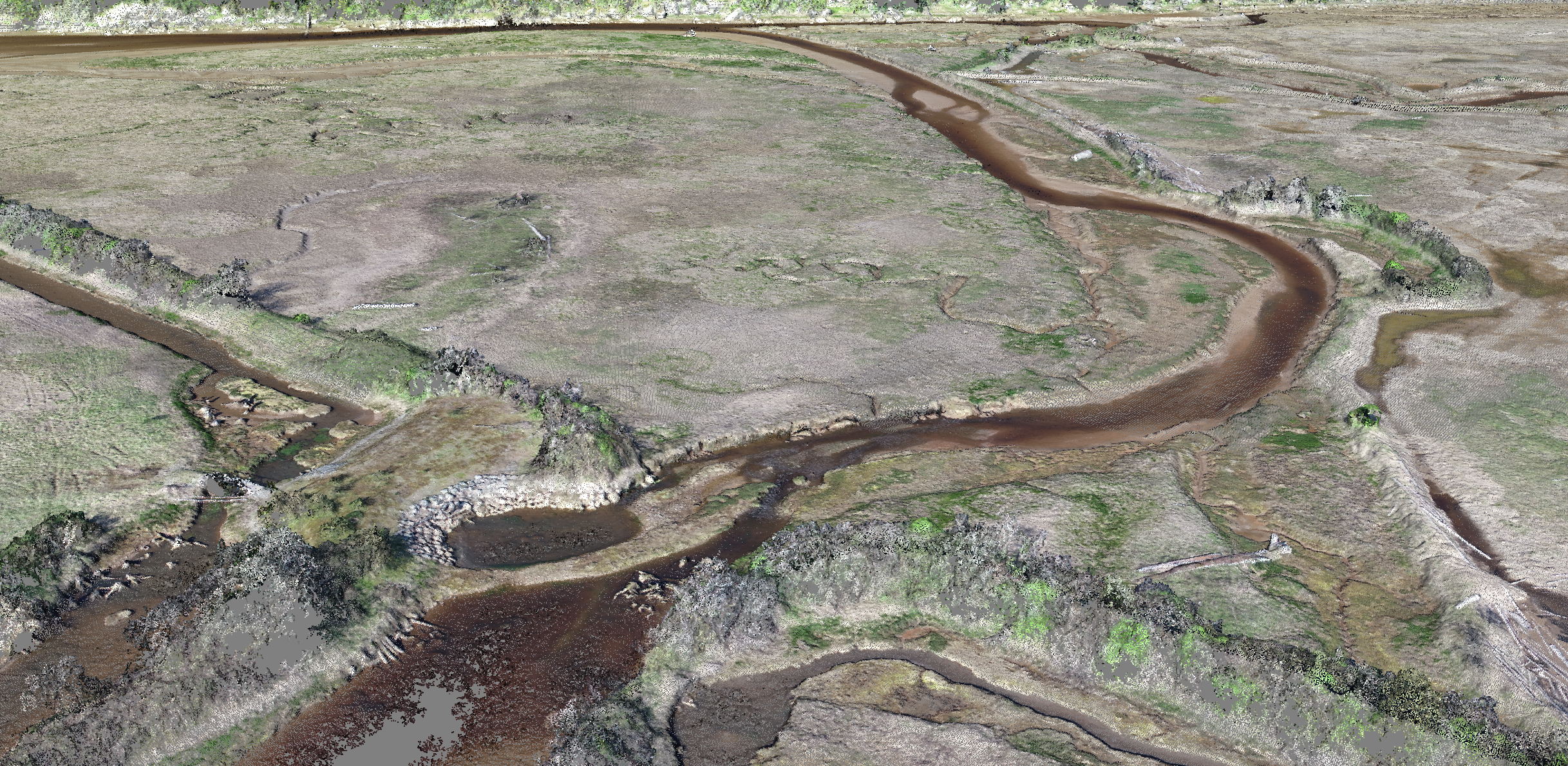
Fine Features - Channels

The high resolution and high precision data produced for this project enable the detection of fine-scale landscape features, like narrow channels. The channel on the left of the above image is 1.6m wide and 60cm deep, while the channel on the right is 0.8m wide and 1m deep. The projected coordinates of the DEM represent the channel bottom very well. These had vertical errors of 6cm and 12cm, respectively. Such a precise model of narrow estuarine channel depth is possible due to the extremely high-density point cloud, which enabled the production of a DEM with accurate projections of confined spaces.

Fine Features - Logs

The dense point cloud also enables the accurate representation of above ground features, such as logs. For example, of the above images the left depicts a large log (4.1m long, 0.8m diameter) that had washed up on the estuarine meadow, with red points indicating GPS validation points (centre and upper-middle of the image). The image on the right is a screenshot of the colourized DEM for the same area. Differences in elevation are clearly visible. These include the light green channel, yellow log and slightly sloping gradient from the top left to the bottom right of the image (from darker to lighter green). The vertical error of the GPS point in the meadow is 6cm, while the vertical error of the point for the surface of the log is 12cm.

The error of both of the previous examples is higher than the average of 4.8cm for the model (9cm average error for the channels, 12cm error for the log). In the case of the channel this is because the channel bottom is visible in fewer overlapping images than the average, providing fewer points of triangulation. The representation of the surface of the log is less precise because it is has a cylindrical shape that is more difficult to reconstruct than a relatively flat surface. A lower altitude flight would be required to increase the accuracy of the reconstruction of this log, but there are few practical reasons to obtain spatial precisions for the height of logs and depth of muddy channels at higher accuracy than was produced here. 

Fine Features - Historic Farm

The meadow areas of the Nanaimo estuary is formerly diked farmland that has since been restored. This area was converted from estuary to farm in the 1800s and was recently restored to an estuarine environment. Visual inspection on-site and from aerial images gives the impression of a uniform meadow, bisected by narrow tidal channels. A visual inspection of the high-resolution DEM makes it immediately apparent that the original farms that used this site have left a lasting impression on the land. These channels, light green lines indicated by white arrows in the above image, show the lasting impression of agriculture on ecologically sensitve sites. 

Interactive 3D Content

Outside of GIS applications, photogrammetric data can be used to allow anyone with access to the internet to explore a conservation site. Photogrammetry can produce 3D models that can be used in the construction of interactive landscape exploration tools. These can be built into customized software applications or presented on web-based applications. We prepared sample 3D content showing recent restoration work (the above image is a screenshot of this). The interactive model can be viewed online at the following link: https://skfb.ly/6yJXo

To view the tour, enter full screen mode. Wait for the image texture to load (this can take a few seconds), then click on the label marked “1.” Then, on the centre bottom of the screen, click the right arrow to move forward through the tour and the left arrow to navigate backward.

Resolution Comparison

The height at which a drone takes pictures has a direct impact on the resolution of orthomosaics. The difference in resolution between flights at 120m and 50m above ground level (AGL) is roughly a factor of three – from 3.1cm/pixel at 120m to 1.2cm/pixel at 50m. The above image compares orthomosaics from images captured at 120m AGL (top) and at 50m AGL (bottom). 

The precision of photogrammetric models is limited to the precision of the GPS points used to construct them. Therefore, reductions in altitude offer increased resolution with limited increases, if any, of geographical precision. While it is possible to construct point clouds of much higher density with flights at lower elevations the practical use of elevation models of landscapes of less than 6cm resolution, such as for DEM produced for the estuary in this project, is limited.

It's important to point out that low-altitude flights work well for open areas but are negatively impacted by areas with trees. Tall trees can create image blur at low altitudes because of their increased proximity to the aerial camera. That is, when camera focus is set for a target (the ground) 50m away tall trees (say, 30m in height) will be out of focus. These trees will also limit the number of ground points captured in their immediate vicinity and their branches can present risks to the drone. Low-altitude flights also take much longer to complete due to the need for high image overlap. For example, a flight at 120m will capture 38,400m2 per image while a flight at 50m will capture 6,700m2. This is 5.7 times less coverage per image, and translates into 5.7 a roughly equivalent increase in flight time and data processing. As a result, low altitude flights are recommended only for open areas when there is a specific need for high-resolution orthomosaics.